
Inferential Statistics for Comparing Means
Assumption of Normality for Statistical Testing:
For Parametric tests which require Normal distribution (approximately) of the sample and population on the test variable. If you run these tests with non normal data:
Power is the probability of rejecting the null hypothesis when in fact it is false. Power is the probability of making a correct decision (to reject the null hypothesis) when the null hypothesis is false. Power is the probability that a test of significance will pick up on an effect that is present.
More Power better the test.
Signal: Numerator
Noise: Denominator
Test Reference: https://libguides.library.kent.edu/SPSS/AnalyzeData
1 Sample T Test
The One Sample t Test determines whether the sample mean is statistically different from a known or hypothesized population mean.
The variable used in this test is known as Test variable
In a One Sample t Test, the test variable is compared against a "test value", which is a known or hypothesized value of the mean in the population.
a 1-sample t-test compares one sample mean to a null hypothesis value. A paired t-test simply calculates the difference between paired observations (e.g., before and after) and then performs a 1-sample t-test on the differences.
The One Sample t Test is a parametric test.
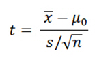
μ = Proposed constant for the population mean
x¯ = Sample mean
n = Sample size (i.e., number of observations)
s = Sample standard deviation
sx¯ = Estimated standard error of the mean (s/sqrt(n))
The calculated t value is then compared to the critical t value from the t distribution table with degrees of freedom df = n - 1 and chosen confidence level. If the calculated t value > critical t value, then we reject the null hypothesis.
EXAMPLES
PROBLEM STATEMENT
According to the CDC, the mean height of adults ages 20 and older is about 66.5 inches (69.3 inches for males, 63.8 inches for females). Let's test if the mean height of our sample data is significantly different than 66.5 inches using a one-sample t test. The null and alternative hypotheses of this test will be:
H0: 66.5 = µHeight ("the mean height of the sample is equal to 66.5")
H1: 66.5 ≠ µHeight ("the mean height of the sample is not equal to 66.5")
where 66.5 is the CDC's estimate of average height for adults, and xHeight is the mean height of the sample.
Examples:
2 Sample T Test
When we want to compare two population means, we used the 2-sample t procedures .
As with the t-test, we can graphically get an idea of what is going on by looking at side-by-side boxplots.
It requires assumption of equal Homogeneity of variances in two samples (i.e., variances approximately equal across groups). You can conduct a test for the homogeneity of variance, called Levene's Test, whenever you run an independent samples t test.
H0: σ12 - σ22 = 0 ("the population variances of group 1 and 2 are equal")
H1: σ12 - σ22 ≠ 0 ("the population variances of group 1 and 2 are not equal")
The data set contains miles per gallon for U.S. cars (sample 1) and for Japanese cars (sample 2); the summary statistics for each sample are shown below.
SAMPLE 1:
NUMBER OF OBSERVATIONS = 249
MEAN = 20.14458
STANDARD DEVIATION = 6.41470
STANDARD ERROR OF THE MEAN = 0.40652
SAMPLE 2:
NUMBER OF OBSERVATIONS = 79
MEAN = 30.48101
STANDARD DEVIATION = 6.10771
STANDARD ERROR OF THE MEAN = 0.68717
We are testing the hypothesis that the population means are equal for the two samples. We assume that the variances for the two samples are equal.
H0: μ1 = μ2
Ha: μ1 ≠ μ2
Test statistic: T = -12.62059
Pooled standard deviation: sp = 6.34260
Degrees of freedom: ν = 326
Significance level: α = 0.05
Critical value (upper tail): t1-α/2,ν = 1.9673
Critical region: Reject H0 if |T| > 1.9673
The absolute value of the test statistic for our example, 12.62059, is greater than the critical value of 1.9673, so we reject the null hypothesis and conclude that the two population means are different at the 0.05 significance level.
To expand it further, if we want to compare ≥ 3 population means.
ANOVA
One-Way ANOVA ("analysis of variance") compares the means of two or more independent groups in order to determine whether there is statistical evidence that the associated population means are significantly different. One-Way ANOVA is a parametric test.
Generally, we are considering a quantitative response variable (which is response "Result" or "Y") as it relates to one or more explanatory variables that are causing value of Y to vary, usually categorical (these are factors such as male/female, various age groups- kids, youngsters, middle aged people, old people).
H0: The (population) means of all groups under consideration are equal.
Ha: The (population) means are not all equal.
(Note: This is different than saying “they are all unequal ”!)
Few examples of this setting:
Which country has the lowest death rate due to Covid-19 Corona virus infection?
Hypothesis:
H0 =
Ha =
What age group has highest infection rate from Covid-19 Corona virus infection?
Hypothesis:
H0 =
Ha =
EXAMPLES
(i) Which academic department in the sciences gives out the lowest average grades? (Explanatory variable: department; Response variable: student GPA’s for individual courses)
(ii) Which kind of promotional campaign leads to greatest store income at Christmas time? (Explanatory variable: promotion type; Response variable: daily store income)
(iii) How do the type of career and marital status of a person relate to the total cost in annual claims she/he is likely to make on her health insurance. (Explanatory variables: career and marital status; Response variable: health insurance payouts)
(iv) Sprint is the respondent's time (in seconds) to sprint a given distance, and Smoking is an indicator about whether or not the respondent smokes (0 = Nonsmoker, 1 = Past smoker, 2 = Current smoker). Let's use ANOVA to test if there is a statistically significant difference in sprint time with respect to smoking status. Sprint time will serve as the dependent variable, and smoking status will act as the independent variable.
Assumption of Normality for Statistical Testing:
For Parametric tests which require Normal distribution (approximately) of the sample and population on the test variable. If you run these tests with non normal data:
- Non-normal population distributions, especially those that are thick-tailed or heavily skewed, considerably reduce the power of the test
- Among moderate or large samples, a violation of normality may still yield accurate p values
Power is the probability of rejecting the null hypothesis when in fact it is false. Power is the probability of making a correct decision (to reject the null hypothesis) when the null hypothesis is false. Power is the probability that a test of significance will pick up on an effect that is present.
More Power better the test.
Signal: Numerator
Noise: Denominator
Test Reference: https://libguides.library.kent.edu/SPSS/AnalyzeData
1 Sample T Test
The One Sample t Test determines whether the sample mean is statistically different from a known or hypothesized population mean.
The variable used in this test is known as Test variable
In a One Sample t Test, the test variable is compared against a "test value", which is a known or hypothesized value of the mean in the population.
a 1-sample t-test compares one sample mean to a null hypothesis value. A paired t-test simply calculates the difference between paired observations (e.g., before and after) and then performs a 1-sample t-test on the differences.
The One Sample t Test is a parametric test.
μ = Proposed constant for the population mean
x¯ = Sample mean
n = Sample size (i.e., number of observations)
s = Sample standard deviation
sx¯ = Estimated standard error of the mean (s/sqrt(n))
The calculated t value is then compared to the critical t value from the t distribution table with degrees of freedom df = n - 1 and chosen confidence level. If the calculated t value > critical t value, then we reject the null hypothesis.
EXAMPLES
PROBLEM STATEMENT
According to the CDC, the mean height of adults ages 20 and older is about 66.5 inches (69.3 inches for males, 63.8 inches for females). Let's test if the mean height of our sample data is significantly different than 66.5 inches using a one-sample t test. The null and alternative hypotheses of this test will be:
H0: 66.5 = µHeight ("the mean height of the sample is equal to 66.5")
H1: 66.5 ≠ µHeight ("the mean height of the sample is not equal to 66.5")
where 66.5 is the CDC's estimate of average height for adults, and xHeight is the mean height of the sample.
Examples:
2 Sample T Test
When we want to compare two population means, we used the 2-sample t procedures .
As with the t-test, we can graphically get an idea of what is going on by looking at side-by-side boxplots.
It requires assumption of equal Homogeneity of variances in two samples (i.e., variances approximately equal across groups). You can conduct a test for the homogeneity of variance, called Levene's Test, whenever you run an independent samples t test.
- When this assumption is violated and the sample sizes for each group differ, the p value is not trustworthy. However, the Independent Samples t Test output also includes an approximate t statistic that is not based on assuming equal population variances. This alternative statistic, called the Welch t Test statistic1, may be used when equal variances among populations cannot be assumed. The Welch t Test is also known an Unequal Variance t Test or Separate Variances t Test.
EQUAL VARIANCES ASSUMED
When the two independent samples are assumed to be drawn from populations with identical population variances (i.e., σ12 = σ22) , the test statistic t is computed as:
with
Where
= Mean of first sample
= Mean of second sample
= Sample size (i.e., number of observations) of first sample
= Sample size (i.e., number of observations) of second sample
= Standard deviation of first sample
= Standard deviation of second sample
= Pooled standard deviation
= Mean of second sample
= Sample size (i.e., number of observations) of first sample
= Sample size (i.e., number of observations) of second sample
= Standard deviation of first sample
= Standard deviation of second sample
= Pooled standard deviation
The calculated t value is then compared to the critical t value from the t distribution table with degrees of freedom df = n1 + n2 - 2 and chosen confidence level. If the calculated t value is greater than the critical t value, then we reject the null hypothesis.
H0: σ12 - σ22 = 0 ("the population variances of group 1 and 2 are equal")
H1: σ12 - σ22 ≠ 0 ("the population variances of group 1 and 2 are not equal")
EQUAL VARIANCES NOT ASSUMED
When the two independent samples are assumed to be drawn from populations with unequal variances (i.e., σ12 ≠ σ22), the test statistic t is computed as:
where
= Mean of first sample
= Mean of second sample
= Sample size (i.e., number of observations) of first sample
= Sample size (i.e., number of observations) of second sample
= Standard deviation of first sample
= Standard deviation of second sample= Mean of second sample
= Sample size (i.e., number of observations) of first sample
= Sample size (i.e., number of observations) of second sample
= Standard deviation of first sample
The calculated t value is then compared to the critical t value from the t distribution table with degrees of freedom
and chosen confidence level. If the calculated t value > critical t value, then we reject the null hypothesis.The Independent Samples t Test is commonly used to test the following:
- Statistical differences between the means of two groups
- Statistical differences between the means of two interventions
- Statistical differences between the means of two change scores
The data set contains miles per gallon for U.S. cars (sample 1) and for Japanese cars (sample 2); the summary statistics for each sample are shown below.
SAMPLE 1:
NUMBER OF OBSERVATIONS = 249
MEAN = 20.14458
STANDARD DEVIATION = 6.41470
STANDARD ERROR OF THE MEAN = 0.40652
SAMPLE 2:
NUMBER OF OBSERVATIONS = 79
MEAN = 30.48101
STANDARD DEVIATION = 6.10771
STANDARD ERROR OF THE MEAN = 0.68717
We are testing the hypothesis that the population means are equal for the two samples. We assume that the variances for the two samples are equal.
H0: μ1 = μ2
Ha: μ1 ≠ μ2
Test statistic: T = -12.62059
Pooled standard deviation: sp = 6.34260
Degrees of freedom: ν = 326
Significance level: α = 0.05
Critical value (upper tail): t1-α/2,ν = 1.9673
Critical region: Reject H0 if |T| > 1.9673
The absolute value of the test statistic for our example, 12.62059, is greater than the critical value of 1.9673, so we reject the null hypothesis and conclude that the two population means are different at the 0.05 significance level.
To expand it further, if we want to compare ≥ 3 population means.
ANOVA
One-Way ANOVA ("analysis of variance") compares the means of two or more independent groups in order to determine whether there is statistical evidence that the associated population means are significantly different. One-Way ANOVA is a parametric test.
- Normal distribution (approximately) of the dependent variable for each group (i.e., for each level of the factor)
- Non-normal population distributions, especially those that are thick-tailed or heavily skewed, considerably reduce the power of the test
- Among moderate or large samples, a violation of normality may yield fairly accurate p values
- Homogeneity of variances (i.e., variances approximately equal across groups)
- When this assumption is violated and the sample sizes differ among groups, the p value for the overall F test is not trustworthy. These conditions warrant using alternative statistics that do not assume equal variances among populations, such as the Browne-Forsythe or Welch statistics (available via Options in the One-Way ANOVA dialog box).
- When this assumption is violated, regardless of whether the group sample sizes are fairly equal, the results may not be trustworthy for post hoc tests. When variances are unequal, post hoc tests that do not assume equal variances should be used (e.g., Dunnett’s C).
Generally, we are considering a quantitative response variable (which is response "Result" or "Y") as it relates to one or more explanatory variables that are causing value of Y to vary, usually categorical (these are factors such as male/female, various age groups- kids, youngsters, middle aged people, old people).
H0: The (population) means of all groups under consideration are equal.
Ha: The (population) means are not all equal.
(Note: This is different than saying “they are all unequal ”!)
Few examples of this setting:
Which country has the lowest death rate due to Covid-19 Corona virus infection?
Hypothesis:
H0 =
Ha =
What age group has highest infection rate from Covid-19 Corona virus infection?
Hypothesis:
H0 =
Ha =
EXAMPLES
(i) Which academic department in the sciences gives out the lowest average grades? (Explanatory variable: department; Response variable: student GPA’s for individual courses)
(ii) Which kind of promotional campaign leads to greatest store income at Christmas time? (Explanatory variable: promotion type; Response variable: daily store income)
(iii) How do the type of career and marital status of a person relate to the total cost in annual claims she/he is likely to make on her health insurance. (Explanatory variables: career and marital status; Response variable: health insurance payouts)
(iv) Sprint is the respondent's time (in seconds) to sprint a given distance, and Smoking is an indicator about whether or not the respondent smokes (0 = Nonsmoker, 1 = Past smoker, 2 = Current smoker). Let's use ANOVA to test if there is a statistically significant difference in sprint time with respect to smoking status. Sprint time will serve as the dependent variable, and smoking status will act as the independent variable.
No comments:
Post a Comment
Thanks for making world's information better and more useful!